Bands, DOS and PDOS: the electronic structure of MgO

In this tutorial you calculate and read the electronic structure of MgO: its band structure along the standard path through the Brillouin zone, its density of states (DOS), the DOS projected on each element and orbital (PDOS), and the band gap. It follows on from Your first calculation, but you can start here.

It takes about 15 minutes; the SIESTA run takes a few seconds.

Before you start

• A SiestaStudio account and SIESTA 5 on your computer (or a cluster).

1. Create a project and load MgO

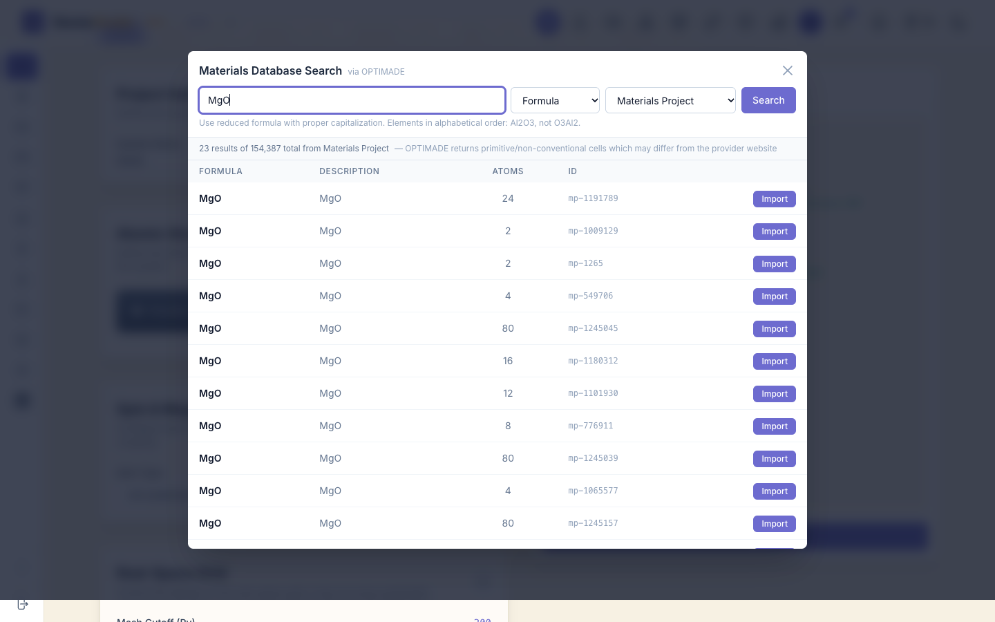
Create a project named MgO bands and open the studio in it. In Atomic Structure, click Search DB, search for MgO and import mp-1265 (rock salt), as in Your first calculation.

2. Set up a band-structure calculation with the wizard

Open the Calculation Setup Wizard and choose Bulk Crystal, Insulator, Band structure and Standard. On the Optional features page, tick Compute DOS. Click Next and Apply All.

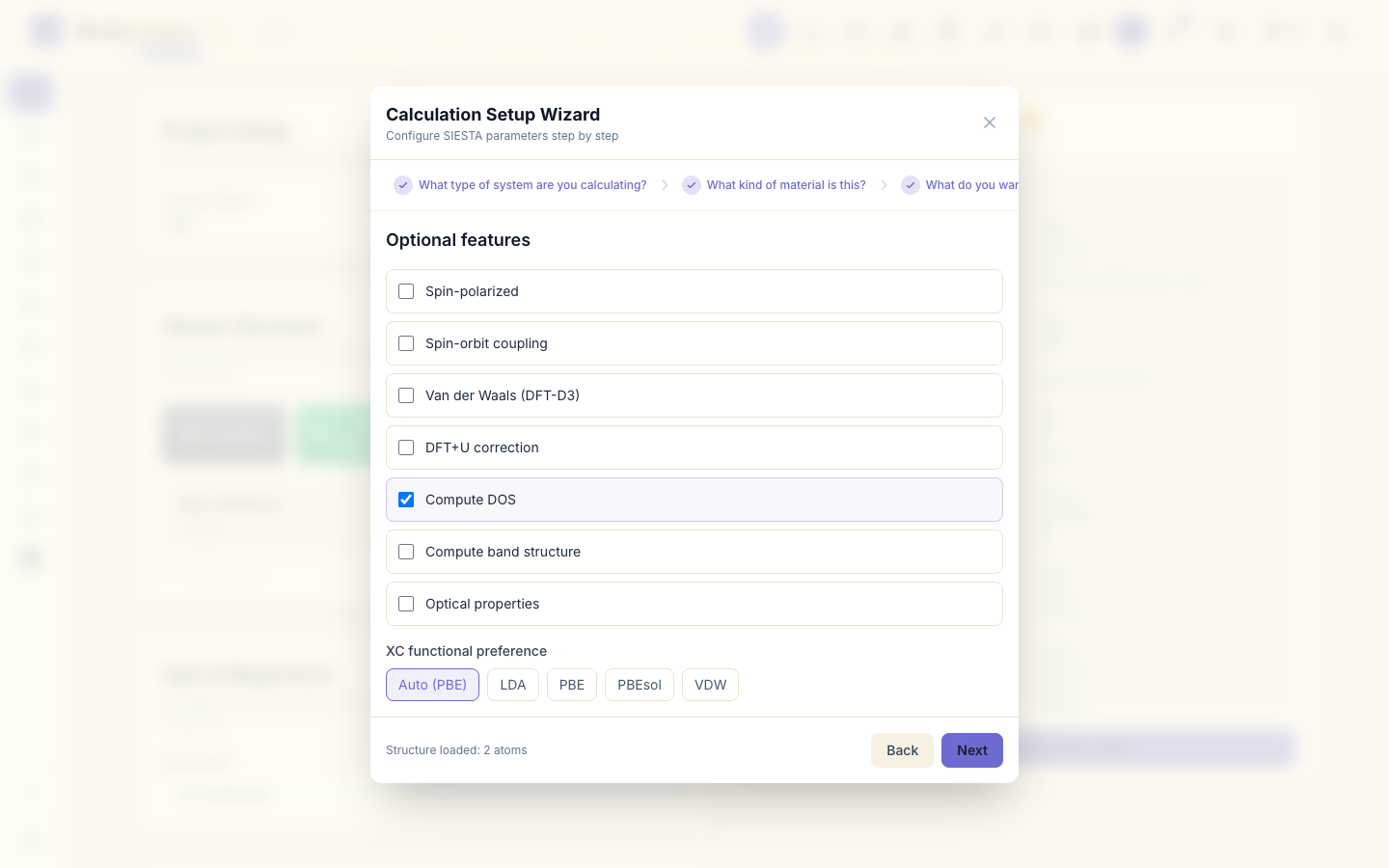
The wizard switches on the band structure, the DOS and the PDOS, but leaves the path through the Brillouin zone empty: you choose it in the next step.

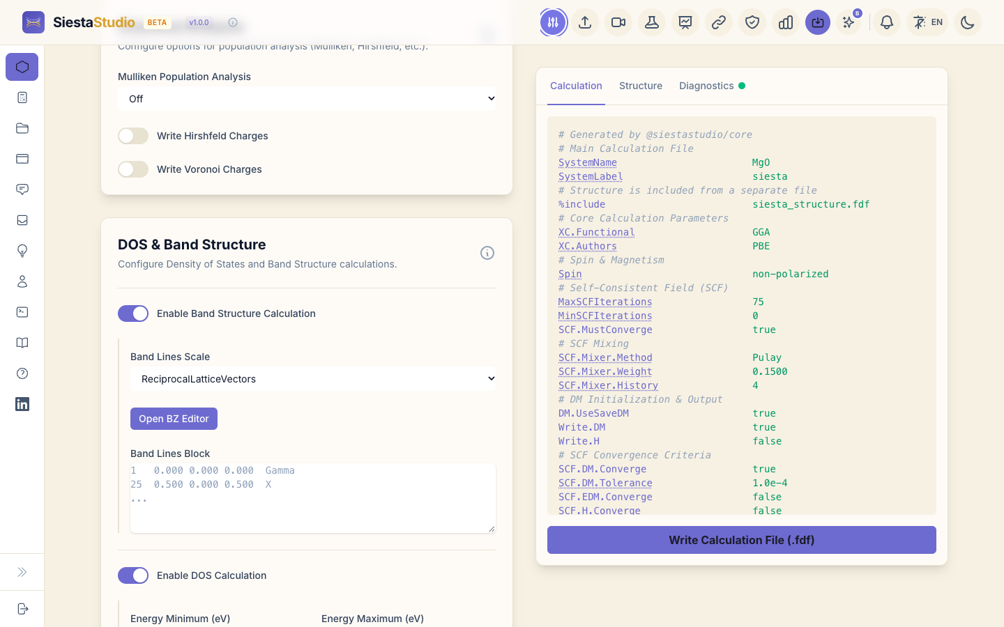
3. Choose the path through the Brillouin zone

In DOS & Band Structure, click Open BZ Editor. The editor recognises the cell as Face-Centered Cubic (FCC), shows its Brillouin zone, and loads the standard path Γ-X-W-K-Γ-L-U-W-L-K-U-X. You can click points in the 3D view to build another path; here the standard one is what you want. Click Apply.

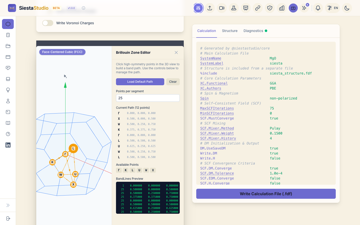
The path now appears in Band Lines Block, one line per point: the number of k-points on the segment that ends there, the point's coordinates in units of the reciprocal lattice vectors, and its label.

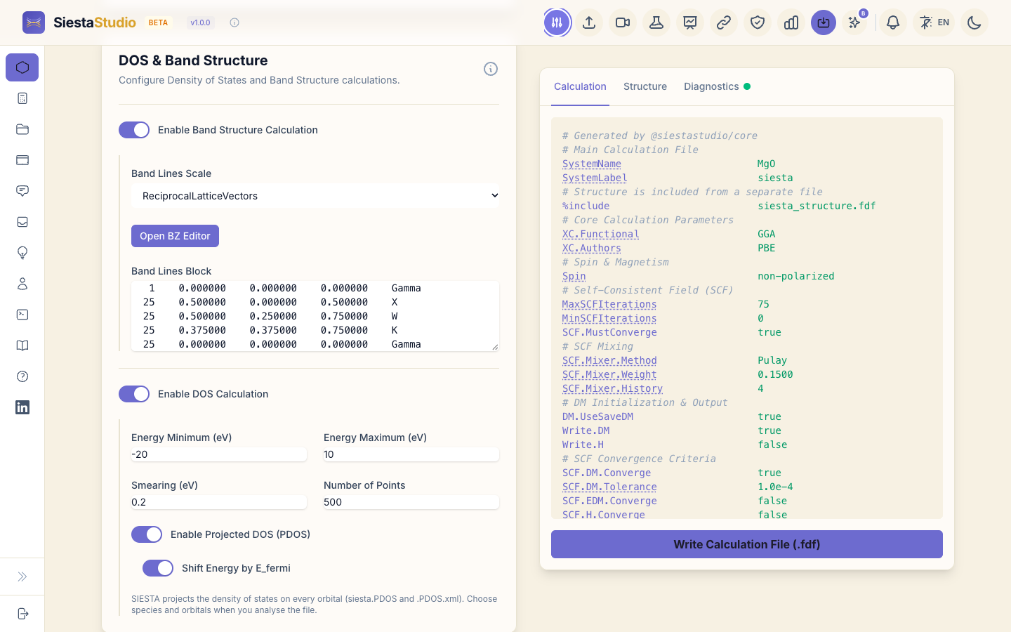
Leave the PDOS Projection Block empty: SIESTA then writes the projections on every orbital, which the studio can sort by element and orbital later.

4. Check, download and save

The Diagnostics tab reports All parameters look good!. Download the two input files (Write Calculation File (.fdf) on the Calculation tab, Write Structure File (.fdf) on the Structure tab) and the pseudopotentials (Pseudopotentials, Download All (ZIP)), and save the calculation to the project.

5. Run SIESTA

With siesta.fdf, siesta_structure.fdf, Mg.psml and O.psml in one folder:

siesta < siesta.fdf > siesta.out

Besides siesta.out, SIESTA writes siesta.bands (the band structure), siesta.DOS (the DOS), siesta.PDOS (the projections), siesta.EIG (all eigenvalues) and Mg.ion, O.ion (the basis orbitals).

6. The band structure

Open Analyze File and drop in siesta.bands. The summary shows 22 bands, the Fermi energy (-2.2629 eV) and the high-symmetry points of the path.

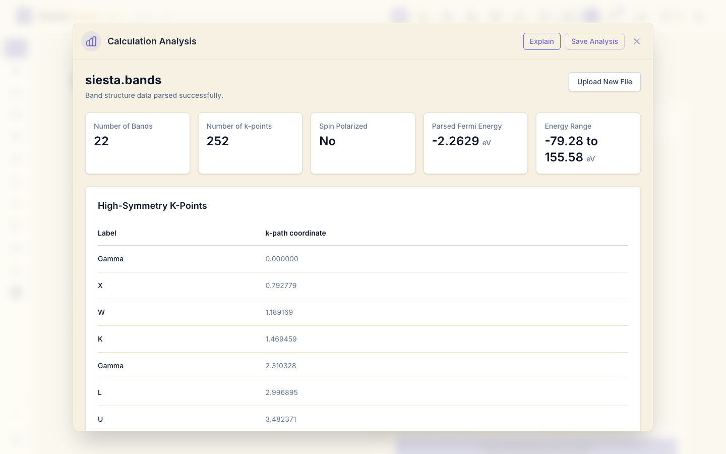
Click Plot Band Structure. The plot first spans every band, from about -80 to +160 eV; set Vertical Min to -15 and Vertical Max to 10 to see the region around the Fermi level (the dashed line at 0).

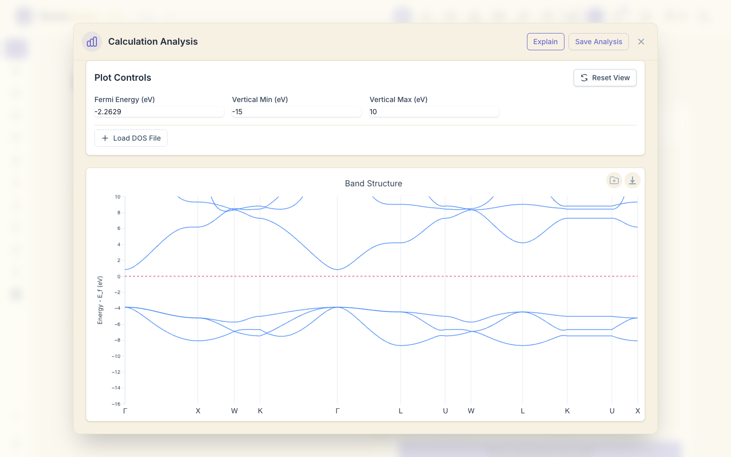
The valence bands (below 0) and the conduction bands (above) are separated by a gap. Both band edges are at the centre of the zone (Γ, the first point of the path and the one between K and L), so MgO has a direct gap.

7. The DOS next to the bands

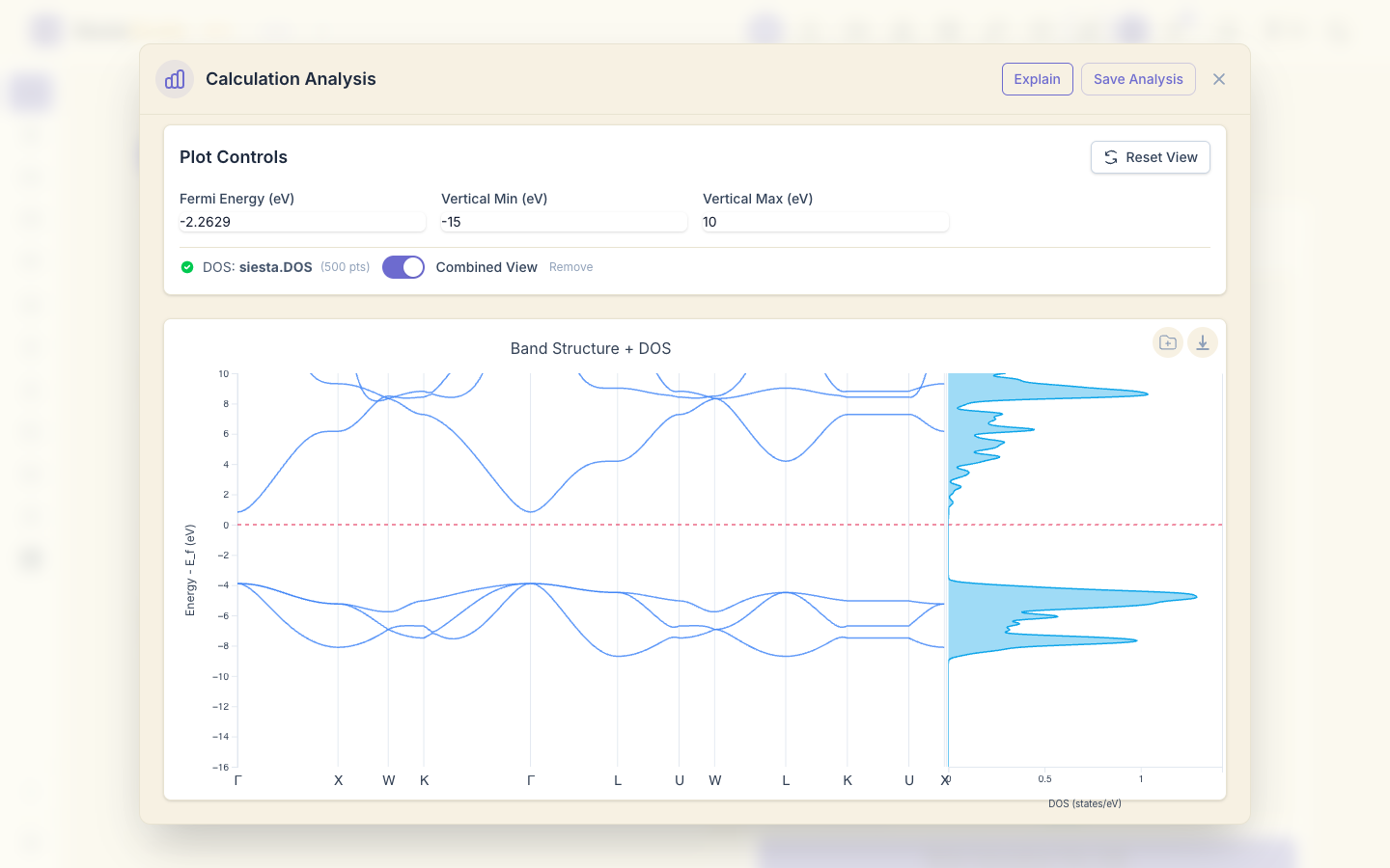
In the band view, click Load DOS File and choose siesta.DOS. With Combined View on, the DOS is drawn beside the bands on the same energy axis: each peak of the DOS is a flat part of a band.

8. The density of states

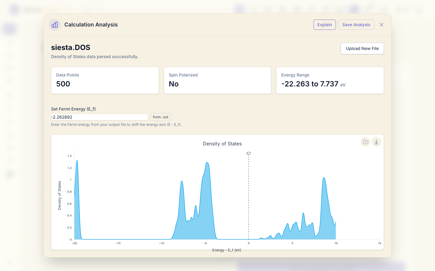
Click Upload New File and open siesta.DOS on its own. A .DOS file holds absolute energies and no Fermi level, so the plot starts on the absolute energy axis. Type the Fermi energy, -2.262892, into Set Fermi Energy (E_f), or click from .out and choose siesta.out, then click Plot Density of States: the energy axis is now relative to the Fermi level.

9. Which atoms and orbitals make each band: PDOS

Open siesta.PDOS. Under By Species tick Mg and O, under By Orbital tick p, and click Plot Selected Projections.

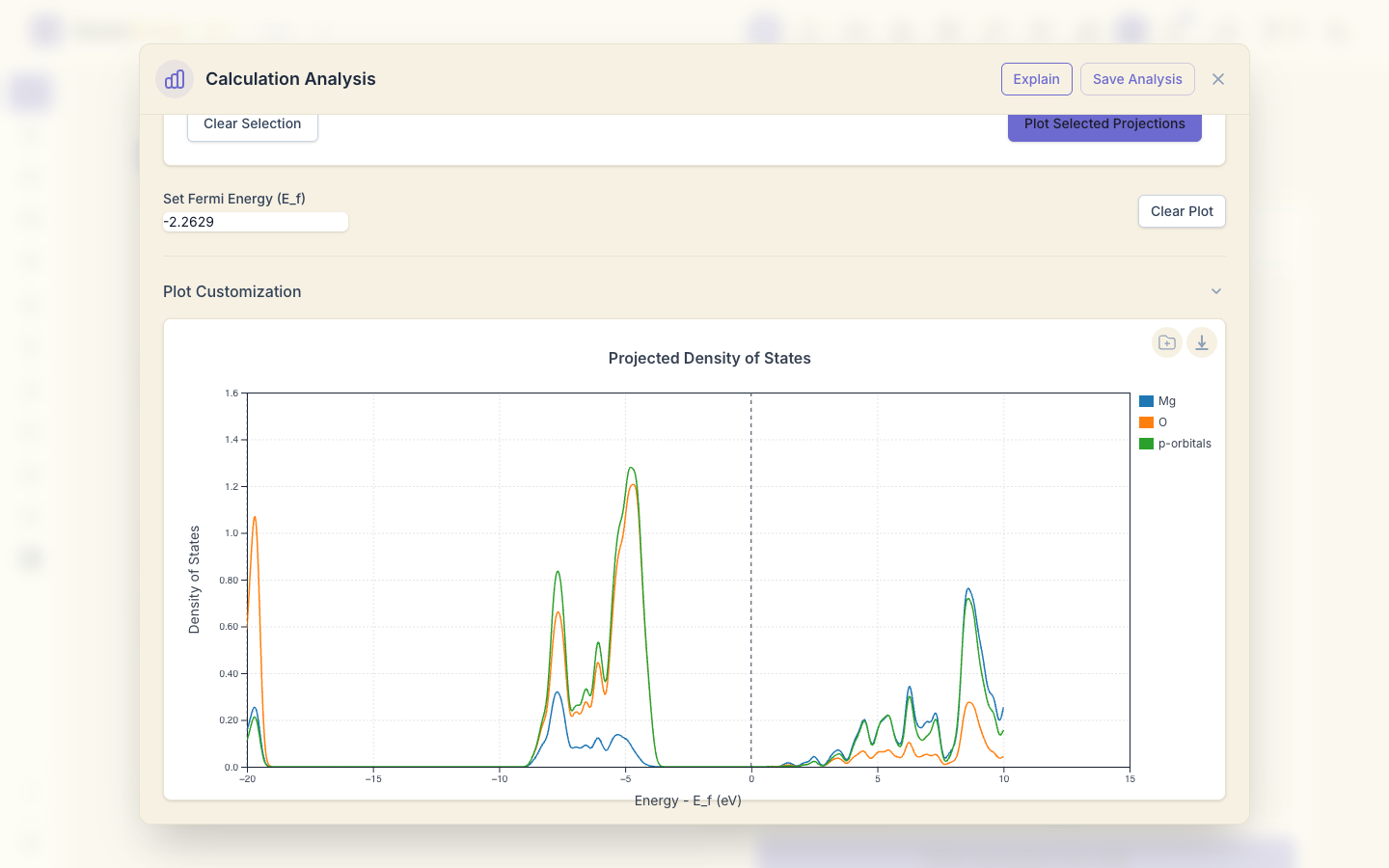
The top of the valence band, about 4 eV below 0 (SIESTA places E_F inside the gap), is almost all oxygen p states: in MgO the valence band is O 2p. The conduction band has more magnesium character. The narrow peak near -19 eV is the O 2s band.

10. The band gap

Open siesta.EIG. The Band Gap card gives the gap, 4.7185 eV, its type, Direct, and the k-point of both band edges.

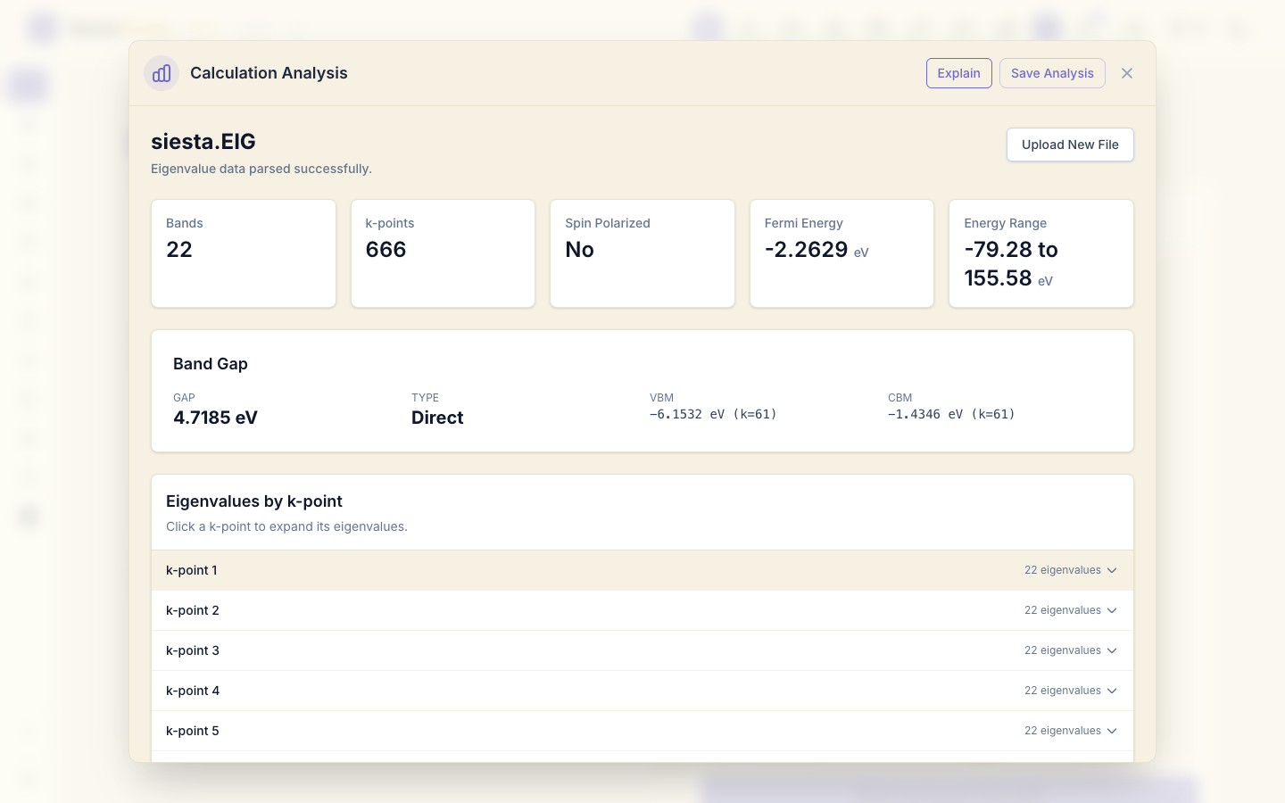
The measured gap of MgO is 7.8 eV. Calculations with GGA functionals such as PBE are known to give gaps well below experiment; the band shapes and the direct gap at Γ are right.

11. The basis orbitals

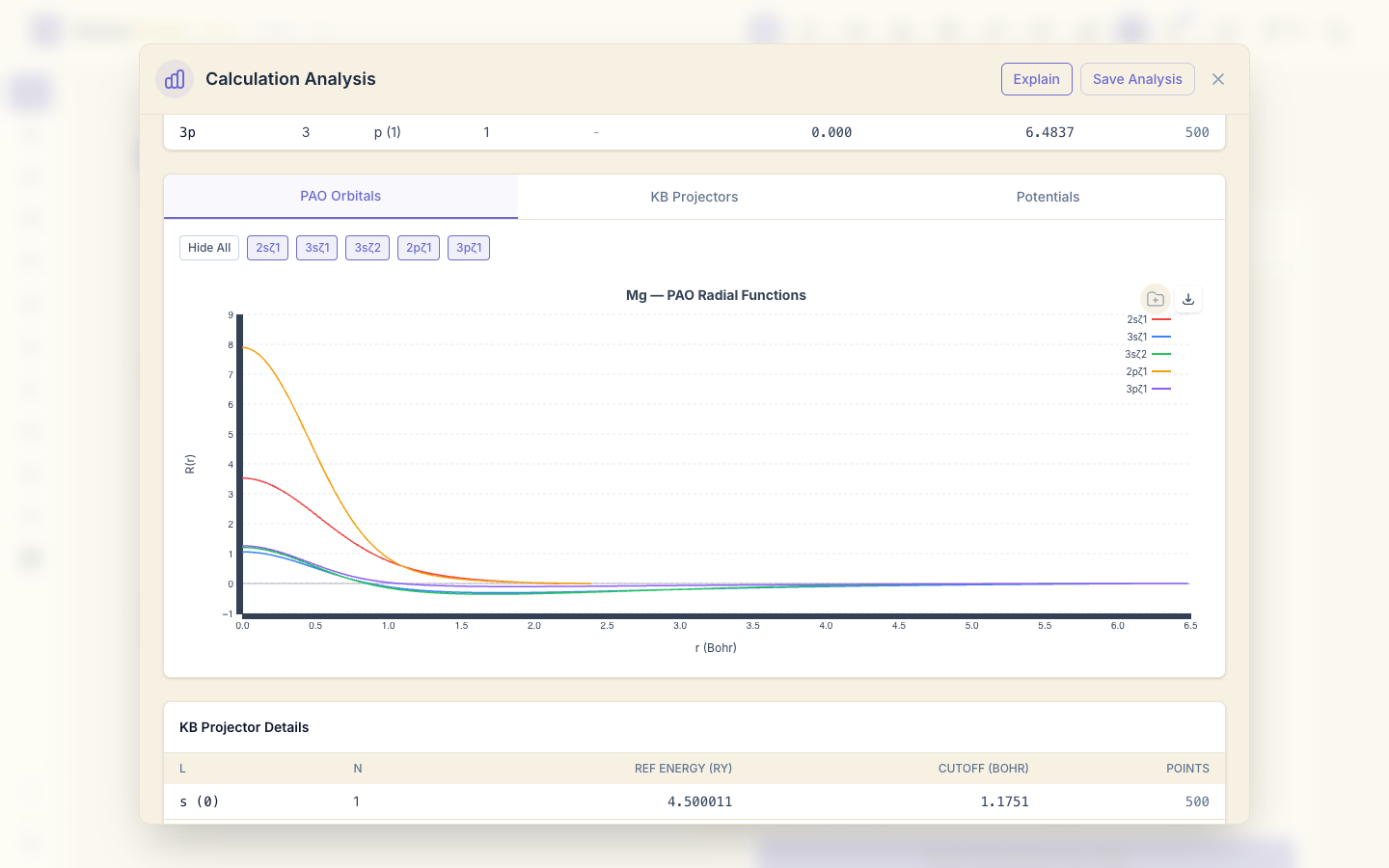
Open Mg.ion to see the numerical atomic orbitals SIESTA used for Mg: their radii, and a plot of each orbital (PAO Orbitals).

12. Save the analysis

Click Save Analysis, choose the project and save.

What next

• Charge density and potential grids: look at where the electrons are.
• Magnetism: spin-polarized bands and DOS of iron.